2D Interpolation, Part 0: The Groundwork

(First of a series) My process for going from a textbook implementation of an algorithm to an efficient production-grade version of it is to methodically apply meaning-preserving transformations that make the code progressively tighter. In this case I'll massage a naïve 2D interpolator that selectively uses nearest-neighbor, bilinear and bicubic interpolation. I started by studying a basic explanation and completed it with the specifics related to bicubic interpolation. Since this is a graphics application, I define meaning-preserving as "agrees on (almost) all pixels", and I carry the test by visual inspection. I use a straight Processing 2 sketch without any complications or embellishments.

To begin with my source data will be a simple 4×4 matrix of floats in the form of an array of arrays with elements repeated around the border. This is not only suboptimal on any number of accounts, it doesn't accomodate the overwhelmingly usual case of image stretching; but for now it is sufficient:

final float[][] data = {
  { 0.60, 0.60, 0.48, 0.24, 0.60, 0.60 },
  { 0.60, 0.60, 0.48, 0.24, 0.60, 0.60 },
  { 0.00, 0.00, 0.36, 0.12, 0.48, 0.48 },
  { 0.24, 0.24, 0.48, 0.60, 0.12, 0.12 },
  { 0.12, 0.12, 0.24, 0.48, 0.36, 0.36 },
  { 0.12, 0.12, 0.24, 0.48, 0.36, 0.36 }
};
final int ny = data.length;
final int nx = data[0].length;

Both bilinear and bicubic interpolation schemes are separable in that they proceed by interpolating by rows first and columns last, in effect composing two 1D interpolations into a single 2D one. In turn, linear and cubic interpolation schemes are expressed as polynomials on an interpolating parameter, t, with coefficients depending on the values being interpolated and obeying certain continuity conditions. These polynomials are standard and derived in a number of places:

static float linear(final float t, final float p0, final float p1) {
  return p0 + t*(p1 - p0);
}

static float cubic(final float t, final float p0, final float p1, final float p2, final float p3) {
  return p1 + 0.5*t*(p2 - p0 + t*(2*p0 - 5*p1 + 4*p2 - p3 + t*(3*(p1 - p2) + p3 - p0)));
}

The functions (ab-)use final and static to convey the impression that they are pure functions (not really, it's just to give HotSpot the chance to inline them). In order to visualize floating-point numbers I use a rainbow palette:

static color hue(float h) {
  final int d, e;
  h = 6 * (h - (float) Math.floor(h));
  e = (int) Math.floor(h);
  h -= e;
  h = (10 - (15 - 6 * h) * h) * h * h * h;
  d = (int) (255 * h);
  switch (e) {
  case 0: return 0xffff0000 |      d  <<  8;
  case 1: return 0xff00ff00 | (255-d) << 16;
  case 2: return 0xff00ff00 |      d;
  case 3: return 0xff0000ff | (255-d) <<  8;
  case 4: return 0xff0000ff |      d  << 16;
  case 5: return 0xffff0000 | (255-d);
  }
  return 0;
}

Why don't I just use Processing's HSB color mode? Two reasons: first and foremost, to use smootherstep to interpolate around the color circle (this eliminates Mach banding and gives prominence to secondary colors); second, so that code that uses it can be made independent of Processing.

The sketch will wait for mouse clicks to react, so the set up explicitly turns off looping:

void setup() {
  size(400, 400);
  noLoop();
}

Every mouse click changes the interpolation scheme in a cyclic fashion:

final static int NEAREST  = 0;
final static int BILINEAR = 1;
final static int BICUBIC  = 2;
int method = 0;

void mouseClicked() {
  method++;
  if (method > BICUBIC)
    method = NEAREST;
  redraw();
}

The sketch will draw directly into the pixels plane, in two passes: the first one will be the current version of the interpolator, and the second will be a baseline version that blacks out identical pixels to highlight differences.

void draw() {
  loadPixels();
  interp0();
  interp1();
  updatePixels();
}

The baseline interpolator, version 0, proceeds in row-major order (first by rows, then by columns) on the destination array pixels to avoid gaps. It calculates (lines 6, 10) the corresponding coordinate in the source matrix as a real (as opposed to integer, not to imaginary), and separates it into an integer part and a fractional part (lines 7–8, 11–12). It then computes an interpolated value from the source data according to method (lines 14–30), computes a color and assigns the pixel (line 31).

void interp0() {
  final float dy = (float) (ny - 3) / height;
  final float dx = (float) (nx - 3) / width;
  int offset = 0;
  for (int i = 0; i < height; i++) {
    float yr = 1 + dy * i;
    int yi = (int) yr;
    yr -= yi;
    for (int j = 0; j < width; j++) {
      float xr = 1 + dx * j;
      int xi = (int) xr;
      xr -= xi;
      float c = 0;
      switch (method) {
      case NEAREST:
        c = data[yi + (int) (yr + 0.5)][xi + (int) (xr + 0.5)];
        break;
      case BILINEAR:
        c = linear(yr,
            linear(xr, data[yi+0][xi+0], data[yi+0][xi+1]),
            linear(xr, data[yi+1][xi+0], data[yi+1][xi+1]) );
        break;
      case BICUBIC:
        c = cubic(yr,
            cubic(xr, data[yi-1][xi-1], data[yi-1][xi+0], data[yi-1][xi+1], data[yi-1][xi+2]),
            cubic(xr, data[yi+0][xi-1], data[yi+0][xi+0], data[yi+0][xi+1], data[yi+0][xi+2]),
            cubic(xr, data[yi+1][xi-1], data[yi+1][xi+0], data[yi+1][xi+1], data[yi+1][xi+2]),
            cubic(xr, data[yi+2][xi-1], data[yi+2][xi+0], data[yi+2][xi+1], data[yi+2][xi+2]) );
        break;
      }
      pixels[offset++] = hue(c);
    }
  }
}

Every destination pixel with coordinate (i, j) maps to a source element (i*(rows - 1)/height, j*(cols - 1)/width) by rule of three. Since the source matrix already has a border the mapping is adjusted by substituting cols = nx - 2 and rows = ny - 2 and adding 1 to the coordinates. The fractional part of each coordinate indicates "how far along" the neighboring pixels the interpolation should go. The comparison is made with this algorithm in function interp1 and where line 31 is changed to:

      if (pixels[offset] == hue(c))
        pixels[offset] = 0xff000000;
      offset++;

The results are:

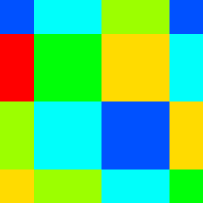
for the nearest-neighbor interpolation,

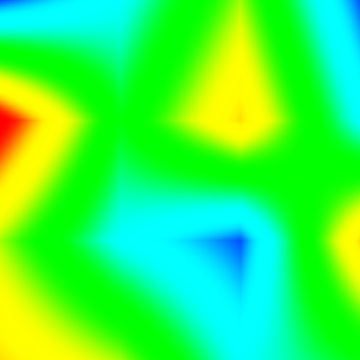
for the bilinear interpolation, and:

for the bicubic interpolation. I know, the colors are toxic. Of course, with the draw() that I've given above the result should be solid black for each mouse click; to see the interpolations in action, comment the call to interp1().

In the next post I'll show a number of massages performed on interp0().